Code Examples of esProc Foreign Key Function

If k (a single field or a combination of fields) is table M’s primary key, and k, at the same time, exists in table B, then k is regarded as B’s foreign key. The foreign key defines a relationship between two tables and is one of the most important concepts for structured data computing. Through object references, esProc makes foreign key easy to function. The following examples aim to illustrate the how foreign key is used in esProc.

Example 1 Associate a referenced table and a referencing table

Order (containing orders information) is the referencing table, emp(containing employee information) is the referenced table. It is required to connect emp with order and display emp’s Name field, Gender field and Salary field and order’s OrderID field and Amount field in the result table.

Note: Besides emp table and order table used here, dep table (containing departments information) is to be used in subsequent examples. The relationship between emp and order/dep through the foreign key is shown as follows: 

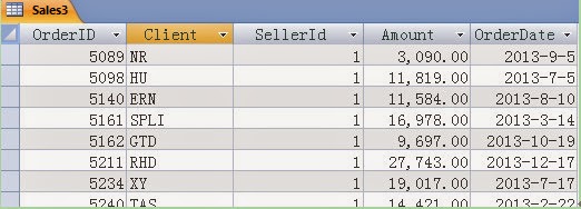
Data may originate from databases or text files. For example:

   order=esProc.query("select OrderID,SellerId,Amount,OrderDate from sales")

   emp=esProc.query("select EId,Name,Gender,Birthday,Dept,Salary from emp")

   dep=esProc.query("select * from department")

esProc code for doing this:

   A3=order.switch(SellerId, emp:EId)

   A4=order.new(OrderID,Amount,SellerId.Name,SellerId.Gender,SellerId.Salary)

Computed result:

Code explanation:

A3: Replace records of order’s SellerID with their corresponding ones in emp to create a foreign key relationship between the two tables. 

A4: Get OrderID field and Amount field from order, and get Name, Gender and Salary field from emp through foreign key references. We can see that, with object references, fields in emp can be accessed directly from order, thus saving us the trouble of writing complex and difficult join statements.

Example 2: Query referencing table according to condition existing in referenced table

Find orders signed by female sellers whose salary is greater than 10,000.

esProc code for doing this:

   A3=order.switch(SellerId, emp:EId)     / the same as above example

   A5=order.select(SellerId.Salary>10000 && SellerId.Gender=="F")

Computed results:

Click the above hyperlinks in blue and corresponding employee information will be shown:

Example 3: Group data according to referenced table

Compute sales amount of each department.

esProc code for doing this:

   A3=order.switch(SellerId, emp:EId)    / the same as above example

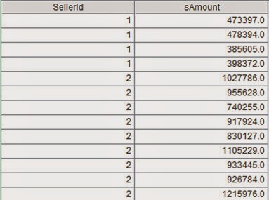
   A5=order.groups(SellerId.Dept;sum(Amount))

Computed results:

You can rename fields, like order.groups(SellerId.Dept:dt;sum(Amount):amt). The effect of name changing is shown below:

Example 4: Complex association between multiple tables

Find managers of departments whose sales amount is greater than 50,000. 

esProc code for doing this:

   A3=order.switch(SellerId, emp:EId)        

   A4=dep.switch(Manager,emp:EId)

   A5=emp.switch(Dept,dep:DeptNo)

   A6=order.groups(SellerId.Dept:dt;sum(Amount):amt)

   A7=A6.select(amt<=50000).(dt).(Manager).(Name)

Computed results:

Code explanation:

A3, A4, A5：Create complete foreign key relationships.

A6: Compute sales amount of each department (See above example). The result is:

A7：Use object references to solve the problem intuitionally. 

Expression A6.select(amt<=50000).(dt).(Manager).(Name) can be divided into four steps according to full stops. They are:

1. Find records whose sales amount is greater than 50,000 from A6.

2. Get records corresponding to those in dt field (from dep table)

3. Get records corresponding to those in Manager field (from emp table)

4. Get Name field.

Details are as follows:

A6.select(amt<=50000)

.(dt)

.(Manager)

.(Name)

An esProc Code Example of Computing Link-Relative Ratio and Year-on-year Comparison

A link-relative ratio is a percentage got by comparing the data of current period and that of the previous period. Usually the interval between the two periods is a month (sometimes an hour, a day, a week and a quarter). The link-relative ratio of April is computed by dividing, for example, its sales amount by that of March. A year-on-year comparison is a comparison between the current period and the same one from the previous year. For example, the comparison between sales amount of April 2014 and that of April 2013. In practical business, data of multiple periods is usually compared in order to find the variation trend.

The inter-row and inter-group computations related to link-relative ratio and year-on-year comparison are common and can be easily handled with esProc. The following example will show you how esProc works.

Case description:

Compute link-relative ratio and year-on-year comparison of growth rate of each month’s sales amount in a specified period. Below is a selection from the Orders table:

esProc code:

A1=esProc.query("select * from sales3 where OrderDate>=? and OrderDate<=?",begin,end)

A2=A1.groups(year(OrderDate):y,month(OrderDate):m;sum(Amount):mAmount)

A3=A2.derive(mAmount/mAmount[-1]:lrr)

A4=A3.sort(m)

A5=A4.derive(if(m==m[-1],mAmount/mAmount[-1],null):yoy)

Code explanation:

A1: Retrieve data from database according to the specified period. begin and end are external parameters. Such as, begin="2011-01-01", end="2014-07-08"(i.e. the data of the current day which can be obtained through now() function). Below is a selection of the query result:

A2: Group orders by the year and the month, and summarize data to get each month’s sales amount. Some of the computed results are as follows:

A3: Add a new field Irr, i.e, the link-relative ratio on a month-on-month basis. The expression is mAmount/mAmount[-1], in which mAmount represents sales amount of the current month and mAmount[-1] represents that of the previous month. Note that value of the first month’s (i.e. January 2011) link-relative ratio is null. Computed results are:

A4: Sort A3 by the month and the year to compute the growth rate of year-on-year comparison. Complete code should be: =A3.sort(m,y). Since A3 has been sorted by the year, so we just need to sort it by the month, that is, A3.sort(m). This has a higher performance. Some of the computed results are: 

A5: Add a new field yoy, i.e., the year-on-year comparison of monthly sales amount. The expression is if(m==m[-1],mAmount/mAmount[-1],null), which means that the comparison can only be made between the same months. Note that the values of year-on-year comparison of months in the initial year (i.e. the year 2011) are always nulls. Some of the computed results are:  

For the convenience of observation, one more line of code, A6=A5.sort(y:-1,m), can be added. That is, sort A5 by the year in descending order and by the month in ascending order. Note that the data ends in July 2014. Results are as follows: 

Grouping In-memory Data Using esProc: Code Examples

Using esProc, it is quite convenient to group data in memory. There are several main types of grouping based on how data is grouped. Here we’ll illustrate equal grouping, alignment grouping and enumeration grouping respectively with an example.

Equal grouping

That data is grouped by one or more certain fields (or one or more computed fields derived from fields) of the current data set is equal grouping. By this method each group is a subset of the original data set.

Case description: Group sales orders by the year.

Data description: The original data is as follow: 

The above data set (table sequence) can be imported from a database or a file. For example:

A1=file("E:/sales.txt").import@t()

esProc code:

A2=A1.group(year(OrderDate))

Computed result:

Code explanation:

1.In this example, the grouping criterion comes from the OrderDate field. The order dates can be converted to the years with year(OrderDate), then data of the same year will be grouped together.

2.There may be more than one field for grouping data. For example, the data could be grouped by both the year and the sellerID to put records of each seller in each year into a group. Below is the code for doing it: A1.group(year(OrderDate),SellerId)

3.Often, the grouped data are to be aggregated, like getting each year’s sales amount based on A2’s data. The code is:

A2.new(year(OrderDate):y,~.sum(Amount):a)

Computed result is as follows:

Or we can combine grouping and summarizing into one step:

A1.group(year(OrderDate):y,~.sum(Amount):a)

Alternatively, we can choose the groups function with better performance yet less flexibility:

A1.groups(year(OrderDate):y; sum(Amount):a)

Of course, sometimes we have to perform grouping and aggregate separately in order to reuse the code and improve computational efficiency, like the scenario in which one of A2’s group needs filtering and another one requires relational computing. In another scenario, the summarized data of a certain group is unusual and worth further study, then this group can be used directly in the subsequent computations without the need of filtering it again.  

4. By default, esProc’s group function will group data using hash algorithm. But for ordered data, the comparison of adjacent rows, which is equivalent to merge operation, may have higher performance. This approach can be implemented by using @o option with group function. For example:

A1.group@o(year(OrderDate),SellerId)

Alignment grouping

Equal grouping groups data by the field(s) coming from within the dataset. If the grouping criterion is one or more fields of another data set, a user-defined array, or a parameter list, etc., the grouping model will be referred as an alignment grouping.

Different from the equal grouping, alignment grouping may produce empty subsets, which means no members in the original data can satisfy a certain grouping condition. It may also lead to incomplete grouping, that is, there may be members that will not appear in any group. Neither would happen with equal grouping. 

Case description: Group the orders table according to the list of best 10 sellers selected by KPIs.

Ungrouped data set:

The orders table in the previous example will also be used here. Data is stored in A1.

The best 10 sellers list is stored in B1 as follows:

The list of sellers may come from an intermediate table, or be generated by a piece of code. It’s not important how it is produced in this example.

esProc code:

A1.align@a(B1:empID,SellerId)

Computed result:

Code explanation:

1. In this example, the grouping criterion (list of sellers) is outside of the data set being grouped. After data is grouped, each group contains only the data of one seller, and groups are arranged according to the order of members in the sellers list. 

2. Because sellers in the orders table outnumber the best sellers, some of the orders will not appear in any group. We can use function option @n to store those orders in one additional group, as shown below:

A1.align@a@n(B1:empID,SellerId)

This group will be put in the end:

3. Sometimes not all members of the grouping criterion will fall in the data set to be grouped. For instance, the grouping criterion is “a list of newly-employed sellers”. In this case, it’s normal to produce empty groups. If we modify the first record of the list into empID=100, the result will be:

Enumeration grouping 

The grouping criterion for enumeration grouping is even more flexible. It could be any boolean expression. The records satisfying the value of the expression will be put into the same group.

Similar to alignment grouping, this is also the incomplete grouping as it probably produces empty subsets or a result in which some members are not included in any group. Moreover, this type of grouping may have the result that certain members appear in more than one group. 

Case description: Dividing orders into four groups, they are: A. order amount is less than 1,000; B. order amount is less than 2,000; C. order amount is less than 3,000; D. order amount is less than 10,000. Special requirement: data cannot be grouped repeatedly, that is, if an order has been in group A, it must not be put into group B, C, or D.

Ungrouped data set:

The orders table in previous examples will still be used. Data is stored in A1.

esProc code:

A2=["?<=1000","?<=2000","?<=3000","?<=10000"]

A3=A1.enum(A2,Amount)

Computed result:

Case explanation:

1. In this example, grouping criteria are multiple flexible expressions. Each record will be compared with each of the expressions. Those records that can match the same expression will be put into the same group. Groups are arranged according to the order of the grouping criteria as well.

2. By default, enumeration grouping will not produce duplicate members in the result. Because after group A’s data is selected out, expression B will be matched with the rest of the records, as this example has shown so far. But the use of function option @r allows us to match expression B with all records, which will produce duplicate members. For example the result of A3=A1.enum@r(A2,Amount) is as follows: 

Likewise, if values of an enumeration expression fall outside of the data to be grouped, it will correspond to an empty group. Besides, if certain records cannot match any expression, function option @n can be used to group these surplus records together. 

esProc Assists Java to Join Text Files

Problem Source: http://stackoverflow.com/questions/26820118/text-file-processing-using-java

JAVA lacks the class library for handling text file JOIN operation. So it’s quite complicated to write code specifically for it, especially when the files are too big to be loaded into the memory all at once. esProc can help JAVA do this kind of operation. Below is an example showing the steps in detail.

order.txt is a text file, in which the first row contains column names and SellerId column is the logical foreign key that points to EID column in employee.txt. It is required to retrieve OrderID, Client, Name and Dept to create a new file. Below are selections of the source data.

Order.txt

Employee.txt

Suppose both files are not big, then we can perform an inner join using the following esProc code:

A1, A2：Retrieve files to memory. @t indicates making the first row as column names.

A3：Perform inner join and the result is as follows:

A4: Retrieve the desired columns from A3.

A5: Export them to a new file. The result is as follows:

If left join is required, then just use @1 option with JOIN function. The code will be =join@1(A1:o,SellerId; A2:e,EId) and the result file is this:

Similarly we can use @f option for a full join.

However if one of the files is big, or both are big, we can handle the operation with esProc cursor. As the following code shows:

A1,A2：Open the big files with cursors.

A3: Inner join of cursors, which, different from the in-memory inner join, requires each cursor is ordered. So sortx function is used here to sort.

A4: Retrieve the desired columns to create a new cursor.

A5: Export the cursor data to a new file.

Similarly, @1 indicates the left join and @f the full join.

So far all the data processing has been done. Then the above script needs to be integrated with JAVA via JDBC, with the following JAVA code:

         // establish a connection via esProc JDBC

         Class.forName("com.esproc.jdbc.InternalDriver");

         con= DriverManager.getConnection("jdbc:esproc:local://");

         // call esProc script whose name is test

         st =(com.esproc.jdbc.InternalCStatement)con.prepareCall("call test()");

         st.execute();//execute esProc stored procedure

         ResultSet set = st.getResultSet();//get the result

esProc Improves Text-processing – Merge Sorted Data

Many databases support the MERGE statement and thus can merge two tables conveniently. Database syntax cannot be used directly, however, if the data to be merged are the text data. In this case esProc is able to perform what MERGE statements can do based on the text files.  

The two files - table1.txt and table2.txt - have the same structure but contain different data. According to the logical primary key defined on column A and column B, table1 will be merged with table2. The operation goes like this: update table1 when the primary key values of the two files are same but values of other columns are different; insert data into table1 when the primary key values are different.

Assume that the original data have been sorted by the logical primary key and make the result set ordered based on the primary key, then you can perform the operation repeatedly and merge new data to the target file.

Below is the original data：

Merge Table 1 with Table 2 and the result is as follows:

esProc code is simple：

A1,B1：Read table1.txt and table2.txt as cursors.

A2：Merge A1 with B1 by the logical primary key. merge function unions data together, ensuring the result set is still ordered. @x represents cursor-handling and @u represents union operation.

A3：Write the result to a new a new file.

Cursor is used in the code to handle data files of any size, even those having big data. 

An Illustration of esProc’s Parallel Processing of Big Text Files

In esProc we can perform parallel processing on big text files conveniently. The following example will illustrate the method.

There is a text file, sales.txt, with ten million sales records. Its main fields include SellerID, OrderDate and Amount. Now compute each salesman’s total amount of big orders in the past four years. The big orders refer to those whose amount is above 2,000.

To do parallel processing, first we must segment the file. esProc provides cursor data object and the related functions to segment and read big text files conveniently. For example file(“e:/sales.txt”).cursor@tz(;, 3:24) means the file is divided roughly into 24 segments by bytes, and the third one will be fetched. Dividing a file simply by bytes will produce incomplete rows, or incomplete records, which need to be processed with additional program. If splitting the file by rows, we have to traverse all the rows while handling one segment of data, which cannot attain a high efficiency expected from parallel processing based on segments. In contrast, esProc automatically rounds off each segment by skipping the incomplete beginning row and completing the ending one, thus ensuring the correctness of the data.

Then we simply need to perform the parallel processing after the file is segmented. Like the following code shows:

Main Program 

A1: Set the number of parallel tasks as 24, that is, divide the file into 24 segments.

A2: Perform multithreaded computation. The tasks are represented by to(A1), whose result is [1,2,3…24], which is the serial number of each segment assigned to each thread. When all the threads complete their computations, the results will be found in A2. B2-B5 is the code within the fork statement.

B2: Read the file with cursor. Which segment should be processed in the current task should be decided according to parameter passed from the main thread.

B3: Select records whose order amount is above 2,000 after the year of 2011.

B4: Group and summarize data for the current segment.

B5: Return the result of the current thread to A2, where the main thread resides.

A6: Merge the results of A2’s multithreading tasks. Below is the selection of the result table:

A7: Group and summarize the merged data to get each seller’s sales amount. The result is as follows:

Code explanation

For the CPU with N cores, it appears natural to set N tasks. The fact is that some tasks always run faster than others, say, according to the differences of filtered data. So the common situation is that some cores are in an idle state after finishing those faster tasks, but a few other cores are still in running with slower tasks. Comparatively, if each core performs multiple tasks in turn, the speed of different tasks will be averaged out and the general operation will become more stable. In the above example, therefore, the task is divided into 24 parts and given to CPU’s 8 cores to process (how many parallel threads are allowed at the same time can be configured in the environment of esProc). But, on the other hand, too many segmented tasks may have weaknesses. One is the decline of whole performance, the other is that there will be more computed results produced by each task when added together, and they will occupy more memory.

fork makes development process simpler by encapsulating complex multithread computation, which enables programmers to focus on business algorithm instead of being distracted by complicated semaphore control.

Computed results of A6 in the above main program have been sorted automatically according to Sellerld, so it is not necessary to sort again in A7 for the grouping and summarizing. @o, the function option of groups, can group and summarize data efficiently without sorting. 

Further illustration:

Sometimes when the data size of a text file amounts to several TB, it is required to use multi-node parallel computation based on a cluster. esProc can perform parallel computation easily. Because its cursor and related functions support non-expensive scale-out file system and distributed file system (DFS). The code will be like this: =callx("sub.dfx", to(A1),A1; ["192.168.1.200:8281", "192.168.1.201:8281", ”......”]). See related documents for detailed usage description. 

Transforming Records with esProc

Problem source：http://bbs.csdn.net/topics/390991336

Table 1 (T1) stores single-value id field and name field. A selection of the source data is as follows:

id    name

1     a

2     b

3     c

4     d

5     e

Table 2 (T2) stores multi-value ids field as follows:

ids

1,2,3

4,3

1,2,3

According to T1’s id field and name field, we want to transform T2’s ids field into a field with values being the corresponding names. The transformed T2 is expected to be like this:

a,b,c
d,c
a,b,c

esProc approach：

A1，A2：Execute SQL statements to retrieve data from T1 and T2.

A3：Convert ids values in A2’s records to sequences one by one, and match them with T1’s records to get sequences of names, which then will be converted to records separated by the comma. The result is like this:

Of course, the above approach is based on the assumption that values of id are consecutive integers. If they are not, then the last step could be rephrased as follows:

  A3：>A1.primary(id)

A4：=A2.(ids.array().(A1.find(~).name ).string@d())

The SQL approach uses subquery to generate distinct group numbers, and then solves the problem with relatively complex JOIN. The following shows how it is coded in MySQL:

  select group_concat(t1.name) names from(

     select @row:=@row+1 as gid,ids from t2,(SELECT @row :=0 ) r

) t2 left join t1 on find_in_set(t1.id,t2.ids) group by t2.gid

But note that this SQL approach can only apply in the situation where there are no duplicate values for ids in T2. Otherwise only one of the duplicates is allowed to be kept. For instance, the transformed result of “2,1,2,3” is “a,b,c” instead of “b,a,b,c”. By comparison, esProc syntax is more intuitive, easier to understand and can be used more widely.

esProc can be called by reporting tools as well as the JAVA program. The way is much like the one a database is called. Through JDBC interface provided by esProc, result can be returned to the JAVA main program in the form of ResultSet. See related documents for detailed method. 

esProc Handles Duplicated Records in CSV files

Problem source：http://stackoverflow.com/questions/28976554/removing-duplicates-from-csv-and-rearranging-the-data-into-columns-with-java

JAVA doesn’t have the class library for grouping data from a text file or getting distinct values, which results rather complicated coding. In dealing with the duplicated records in a CSV file, esProc can work with JAVA to make it easier. The following example will tell you how esProc works.

dup.csv contains 8 columns, in which there are some duplicated values, as shown below: 

We need to filter away the duplicated records, get the first 6 columns and rearrange the 7^th and the 8^th column, according to the rule that work phone will be made the 7^th column and work email the 8^th column for the new file, and if there is more than one work phone or work email for the same person, the first one will be used.

esProc approach：

A1: Import the file separated by commas.

A2: Filter records to remove the duplicated ones and rearrange them. group function is used to group them. ~ represents each group of records; _1,_2…_8 are default column names; @1 indicates getting the first record from the query result. The result is as follows:

A3: Export the result to a new CSV file. Or we can use exportxls function to export data as the Excel format.

Having done all data processing, the esProc script will then be integrated with JAVA program via JDBC using the following JAVA code:

         // establish a connection via esProc JDBC

         Class.forName("com.esproc.jdbc.InternalDriver");

         con= DriverManager.getConnection("jdbc:esproc:local://");

         // call esProc script, whose name is test and which receives parameters

         st =(com.esproc.jdbc.InternalCStatement)con.prepareCall("call test()");

         st.execute();//execute esProc stored procedure

         ResultSet set = st.getResultSet();//get the result

esProc Counts Distinct Columns in a Text File

Problem source：http://unix.stackexchange.com/questions/161885/using-awk-to-identify-the-number-identical-columns

There are some text files under /data directory. Each of them has certain columns. We want to know how many distinct columns are there in each file. For instance, the number of distinct columns in f1.txt is 3. 

Suppose there is only one file. Then the code could be:

file("/data/f1.txt”).import().fno().((c=#,A3.(~.field(c)))).id().len()

fno function is used to get the number of columns in a two-dimensional table; ~ represents the loop variable of a loop function; # represents loop number; and id function is used to get the distinct columns.

If there are a great number of files under /data directory, the code will be more complicated:

pjoin((d=directory@p("/data")),d.((f=file(~).import(),f.fno().((c=#,f.(~.field(c)))).id().count())))

This line of code calculates sequentially the number of distinct values in each file and joins the results with corresponding file names. The result table is as follows:

For the convenience of observing computational logic, the above code can be written in multiple cells using a long statement:

== indicates the beginning of the long statement, whose working range is the indented block of B2-C5. B5 is the last executable cell whose result will be returned to A2. 

esProc Assists BIRT to Dynamically Insert Subtable Fields into Primary Table

Database table dColThread is the primary table with the primary key tID. dColQuestion is the subtable with the foreign key tID, as shown in the following figures:

dColThread

dColQuestion

The desired report will display data in the grid in which the primary table is presented according to ApplicationName. Each record in the primary table may correspond multiple, yet not greater than five, status values. These values need to be inserted between the primary table’s Phone field and Decline field in five columns that are named QuestionNo1, QuestionNo2…QuestionNo5 respectively. If one of these columns is empty, then hide it. The appearance and layout of the report is as follows:

Prepare the necessary data in esProc using the following code：

A1：Execute the SQL statement to retrieve data from the two associated tables – the primary table and the subtable. arg1 is a report parameter. Suppose arg1=“mfc”, then A1’s result is as follows:

A2：Group A1’s table by tID. Each group includes a record of primary table and its corresponding records from the subtable, as shown in the figure below:

A3：Create an empty two-dimensional table according to the data structure of the report table.

A4：Loop through A2’s groups and insert values into a record of A3 with each loop. In the loop body, A4 is used to reference the loop variable and #A4 is used to reference the loop number.

B4：Get status values of the current group and append to at least five columns.

B5：Append new records to A3. When the loop is over, A3’s table is as follows:

A6：Return A3’s result to the report. esProc provides JDBC interface and it will be identified by reporting tools as a database.

Then design the grid report in BIRT. The template is as follows:

We need to hide a QuestionNo column if it is empty. There are many approaches to dynamically hide it. Here is one of them. To hide column QuestionNo5, we can use the following script (also applicable to other columns) in dataSet’s onFetch method:

if(reportContext.getGlobalVariable("t5")==null){

    reportContext.setGlobalVariable("t5",row.QuestionNo5)

}else{

    reportContext.setGlobalVariable("t5",reportContext.getGlobalVariable("t5")+row.QuestionNo5)

Then use the expression BirtStr.trim(reportContext.getGlobalVariable("t5"))=="" on column QuestionNo5’s Visibility property.

A preview of the final report is as follows:

The way a report calls the esProc script is the same as that it calls the stored procedure. Save the above script as dColMiddle.dfx, which can be called by call dColMiddle.dfx(?) in BIRT’s stored procedure designer.