esProc Finds Differences between CSV files

userName and date are the logical primary key of both old.csv file and new.csv file, in which we want to find rows that are new, deleted and updated.

The source data is as follows:

As can be seen from the above data, in new.csv the 2^nd and the 3^rd row are the new and the 4^th row is the updated; in old.csv the 3^rd row is the deleted.

esProc code：

A1,B1：Retrieve the comma-separated files.

A2,B2：Sort data by the key, as this is required by the following merge function.

A3：Find the new records by the key. merge function is used to merge data sets. @d means calculating the difference during the merge. Similar options include @u for union and @i for intersection. The computed result is as follows:

A4：Find the deleted records by the key. The computed result is as follows:

A5：Take the key fields as ordinary ones to find the updated records. The computed result is as follows:

A6：A5 is an intermediate result. We need to calculate the difference between A5 and the new records to get the updated records. The computed result is as follows:

B6：Return A6 to JAVA program or the reporting tool.

Now all data processing work has been finished. We’ll then integrate the esProc script into JAVA program via JDBC. The JAVA code is as follows:

  //establish a connection via esProc JDBC

  Class.forName("com.esproc.jdbc.InternalDriver");

  con= DriverManager.getConnection("jdbc:esproc:local://");

  //call esProc script, whose name is test and that can accept parameters

  st =(com.esproc.jdbc.InternalCStatement)con.prepareCall("call test()");

  ResultSet set = st.getResultSet();//get the result

If you want to return multiple data sets to the JAVA program, you can modify B6’s code into result new,delete,update. 

Index Performance Comparison between Oracle and esProc

Data table indexing is a common method to accelerate query in Oracle. esProc also provides indexing function. With the actual measurements in the several examples below, we can compare their speed after indexing.

The test is performed on data table T3 with 165 million records. The binary data file being saved in esProc format takes up 14.6G physical storage,in which fields are shown below:

CREATE TABLE "T3"

   ( "L11" NUMBER(11,0),

         "L4" NUMBER(9,0),

         "D4" VARCHAR2(9),

         "C4" VARCHAR2(10),

         "R2" DATE,

         "R4" DATE,

         "FL6" NUMBER(9,0),

         "FD6" VARCHAR2(6),

         "FC6" VARCHAR2(9),

         "TL1" NUMBER(2,0),

         "TL11" NUMBER(7,0),

         "TN1" NUMBER(5,2),

         "TN11" NUMBER(23,2),

         "TN21" NUMBER(9,2),

         "TN31" NUMBER(9,2)

   )

Provide the same hardware for both Oracle and esProc with the below environment configuration:

Model for test: Dell Power Edge T610

CPU: Intel Xeon E5620*2

RAM: 20G

HDD: Raid5 1T

Operating system: CentOS 6.4

JDK: 1.6

Oracle version: 11g

esProc version: 3.1

1.   Indexing Performance Comparison

4 indexes have been created for both Oracle and esProc. The first 3 are the single-field indexes, and the forth index is the composite indexes.

Note: The test results in this article are all represented in seconds unless otherwise remarked.

As can be seen from the above figure, indexing in Oracle is faster than that in esProc. The main application scenario of esProc is the data computing in BI. In this sector, the data seldom changes. Owing to this, the comparatively slow speed is acceptable since indexing can be regarded as a one-off job.

2.Single-field Indexing Performance Comparison

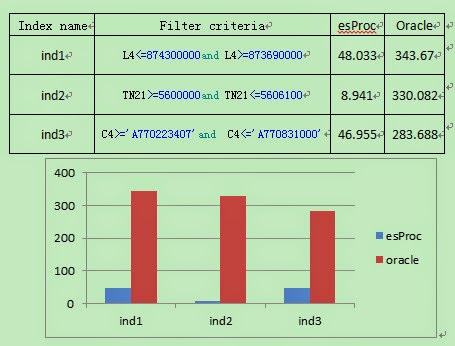
In below discussion, let’s compare the query speed between Oracle and esProc. To start with, let’s compare three single-field indexes. In which, the ind1 is the single-field index for the integer field L4; the ind2 is the single-field index for real number field TN21; and the ind3 is the single-field index for the character field C4. Compare the respective time consumed to query based on filtering criteria.

2.1. Less than 10 records satisfying the query conditions

As can be seen from the above figure, compared with Oracle, esProc is faster in handling the integer field, comparable in handling the real number field, and slower in handling the character field.

2.2.  Around 100 records satisfying the query conditions

As can be seen from the figure, esProc is relatively faster for the numeric field, and the speeds of esProc and Oracle in handling the character field are close.

2.3.  Around 10000 records satisfying the query conditions.

As can be seen from the above figure, esProc runs faster, but the difference is not great.

2.4.  Around 100000 records satisfying the query conditions

As can be seen from the above figure, esProc runs faster, demonstrating its obvious advantages.

3.   Multi-field Composite Indexing Performance Comparison

3.1.  Less than 10 records satisfying the query conditions

As can be seen from the above figure, Oracle performance is better.

3.2.  Around 100 records satisfying the query conditions

As can be seen from the above figure, Oracle performance is relatively better if there are around 100 records satisfying the conditions.

3.3.  Around 10000 records satisfying the query conditions.

As can be seen from the above figure, esProc performance is obviously superior when the composite indexes of the 3 fields are all the filter criteria and there are 10000 records satisfying the condition.

3.4.  Around 100000 records satisfying the query conditions

As can be seen from the above figure, esProc performance is better if there are 100000 records satisfying the condition.

4.   Findings on Performance Comparison

1. Indexing in Oracle is several times faster than that in esProc. Comparatively, esProc more fit for the BI data computing. In most BI scenarios, relatively few data changes, and indexing can be regarded as a one-off job. A bit slowdown in speed is also acceptable.

2.After indexing, in case a small number (<10000) of records satisfy the query conditions, Oracle is often superior to esProc; In case the number of records is at a medium level (>10000,<100000), their performance is close; In case a great number of records (>100000) return, esProc demonstrates an obvious performance advantage.

Comparison between esProc Syntax and SQL Syntax for Common Computations

Structured Query Language, abbreviated as SQL, is usually used to query, store and retrieve data in databases. In esProc, users can return the query result using SQL commands directly, or process data step by step with more flexible and convenient methods and get the same result as that of SQL, whose computation is complicated.

1. esProc syntax and SQL syntax for common computations

1.1 Select the specified fields

With T.new() function, specified fields can be selected from the pre-existing table sequence T to create another table sequence. Actually, an SQL statement is usually used directly to select the specified fields if other fields of the data table aren’t needed. Results in A2 and B2 are the same:

1.2 Filter records with “where” 

With T.select() function, specified records can be selected from table sequence T to create a record sequence. In both A2 and B2, data of states where population is greater than 15,000,000 are selected, and the results are the same:

1.3 Remove duplicates with “distinct”

 

With T.id() function, the result, in which duplicates have been removed, can be obtained from table sequence T. In both A2 and B2, the serial numbers of states, in which cities listed in table CITIES are located, can be viewed. The results are the same:

1.4 Sort with “order by”

With T.sort() function, the records in table sequence T can be sorted and a new record sequence will be returned. In A2 and B2, data are sorted by city names in ascending order:

In A3 and B3, data are sorted by city names in descending order:

1.5 Group and summarize with “group by” 

The SQL statement in A2 groups the cities and counts the cities which each state has in the table CITIES. The result is as follows:

In B2, groups function is used in esProc to group and summarize the data of the table sequence. The result is as follows:

The summarizing results obtained by using both methods are the same. The only difference is that data are automatically sorted in esProc according to the grouping criteria during the process of grouping and summarizing.

1.6 Foreign keys 

In databases, the relationship between two tables is usually represented by the foreign key. For example, relate the table of cities information –CITIES - to table of states information –STATES - by field STATEID of the former table. In order to show the computational method of the relating, only the data of states whose serial numbers are less than 10 are selected. Since a statement is needed to get the result when SQL is used to perform a task, methods like nested SQL, whose statements are complicated and unreadable though, are required. While in esProc, a step-by-step method is adopted: fetch data with B1 and B2; use switch function in B3 to connect data of the two tables. As shown below, the table sequence is changed in B1:

It can be seen that the data of field STATEID are set to correspond to the state records. Seen from the computation in B4, the value of fields of record type can be called conveniently, as the abbreviations of states are obtained using STATEID.ABBR. Then, the result in B4 is the same as that in A4:

1.7 Join multiple tables together with “join” 

The SQL statements used in A3 and A4 are inner join, but they have different syntax. When the data of two tables are being joined, only the data that have inter-table relations with each other will be fetched. The returned result in A3, A4 and B3 are all the same. Note that the order of records in the results returned by SQL and esProc respectively may be not the same:

The SQL statement in A5 is a left join. When the data of the two tables are being joined, besides the data that have inter-table relations with each other, all the unrelated data in the first table will also be fetched. This means, in the result, field STATE may be null and field CITY won’t be null. This case, in fact, is the foreign key relationship. To join tables together in esProc, both switch and join@1() function, in which the 1 in @1 option is a digit, can be used. Letter l won’t appear in esProc options for fear of confusion. The returned results in A5 and B5 are the same. As the above, the order of records in the results returned by SQL and esProc respectively may be not the same:

The SQL statement in A6 is a full join. When the data of the two tables are being joined, all data of both tables after relating will be fetched, meaning both of the two fields: STATE and CITY, in the result may be null. The operation can be performed with join@f() function in esProc. The returned results in A6 and B6 are the same but the order of records in them may be different:

The SQL statement in A7 is a right join. When the data of the two tables are being joined, all the unrelated data in the second table, besides the data that have inter-table relations with each other, will be fetched. This means, in the result, the field CITY may be null but field STATE won’t be null. Without a similar usage, esProc needs to switch the positions of the parameters in join@1(), the left join function, to complete the same operation. The returned results in A7 and B7 are the same though the order of records in them may be different:

1.8 Union the results with “union” 

union all or union can be used in the SQL statements to union the data from two result sets. But in esProc, two sequences can be concatenated to merge the data from two result sets completely. The results in A3 and B3 are the same:

merge@u() function can be used in esProc to remove the duplicates in the result. The results in A4 and B4 are the same:

Only the first of the two duplicate records of Los Angelesin the previous resultis kept.

2 esProc functions and SQL functions

We can use various functions in the SQL statements. But different databases require different syntax. For example, TODAY() is the standard SQL function to get the current date, but SYSDATE should be used in Oracle and GETDATE() is required in the SQL Server. This is so complicated. However, the trouble brought in by different syntax can be avoided if the data can first be fetched in esProc and then be processed as required.

2.1. Logical judgment

The operators for logical judgment used in esProc are similar to those used in high-level programming languages, like Java. But they are different from the SQL operators of the same use:

In SQL, “=”is used to judge if two things are equal, “OR” to represent the “OR operation” and “AND” to represent the “AND operation”. While in esProc, the double equals “==” is used to judge if two things are equal,“||”to represent the “OR operation” and “&&” to represent the “AND operation”.

In A2 and B2, the records of cities, in which the value of field STATEID is 5, are selected:

In A3 and B3, the records of cities, in which the value of field STATEID is 5 or 13, are selected:

In A4 and B4, the records of cities, in which the value of field STATEID is 5 and the value of POPULATION is greater than 1,000,000, are selected:

2.2 String functions

The usage of string functions in esProc is similar to that of standard functions in SQL, for example:

The usages of left function in A2 and B2 are completely the same. But to get cities whose initials are F, the string is single-quoted in the SQL command while it is double-quoted in the esProc expression:

The string functions that have similar syntax include right/mid/replace and so on. In addition, the usages of mathematical functions like abs/ceil/round/floor/sin/cos/tan/power/sqrt in SQL and esProc are basically the same.

The names of some corresponding functions are different in SQL and in esProc. For example, the function for returning the length of a certain string is length in SQL while its counterpart in esProc is len. In A3 and B3, the cities whose names are composed of four letters are selected:

And the usages of some functions are also different in SQL and in esProc. For example, keyword like is used in SQL to judge if a string is of the specified format while like function is used in esProc to do the same thing. The cities starting with a C and ending with an e are listed in A4 and B4:

To concatenate strings, concat function is used in SQL, while a “+” can be used directly in esProc though the digits should be converted into the string first. The results in A5 and B5 are the same:

2.3 Date/time functions 

All the common date/time functions in SQL can find their counterparts in esProc and their usages are similar. For example, the year function for getting the year value in A3 and B3. Similar functions include month/day/hour/minute/second and etc. The data of employees who were born in 1980 are fetched in both A3 and B3:

esProc boasts some easy-to-use functions SQL hasn’t. For example, age function is used in B4 to compute the ages of employees in the result. But the same computation is difficult to perform in SQL. The result in B4 is as follows:

2.4 Summary functions

The usages of common summary functions, such as count/sum/avg/max/min, are the same in esProc and in SQL. The results in A2 and B2 are the same, but the data in B2 have been sorted by grouping conditions: